When we are programming and we type something in our IDE, for example, User.where( and we see the “editor” suggests method names to complete our code, this is not AI, this is the IDE following some rules, but when we type the same and Claude or Github Copilot suggest a whole implementation of a method using it, or when Gemini creates an entire test suite from our requirements, that’s an LLM (Large Language Model)!

In this post, you will learn all the basics behind LLMs, such as Machine Learning, Deep Learning, Neurons, and Neural Networks. First, I will introduce the fundamental concepts underlying large language models. Next, we will explore the structure and processes of machine learning and deep learning, including key components such as neurons and neural networks. Finally, the goal of this first post in the series is to build our first neural network in Ruby, setting the foundation for subsequent posts where we will implement AI features in Rails applications.

Let’s start by understanding what makes LLMs possible.

What are LLMs, and what makes them possible?

A Large Language Model (LLM) is a type of AI program trained on large amounts of data or examples, enabling it to understand human language and generate coherent text responses or other complex data, such as images or video. Unlike traditional programs like our IDE, LLMs learn patterns from millions of examples:

Predict the following sentence when you are writing an email.
Understands different languages in the same context.
Suggests an entire code block based on context.
Generates tests for your code based on the logic you wrote.

That’s possible because LLMs are built using Deep Learning, a specialized subset of Machine Learning. More specifically, they use a deep learning architecture known as a transformer model.

Here’s the accurate hierarchy:

Machine Learning (learning from data)
- Deep Learning (subset using multi-layered neural networks)
  - Neural Networks (Processing data through layers and neurons)

But don’t worry, we are gonna explain all these concepts 👌. We’ll start with Machine Learning, continue with Deep Learning, explore neurons, and finally build a simple neural network in Ruby. By the end, you’ll understand the base that makes LLMs possible.

Machine Learning

It’s a branch of AI focused on algorithms that can “learn” patterns from training data, enabling machine learning models to make predictions without specific instructions. For example, we have a model that finds only sports cars. It may start by identifying any vehicle, but after being fed with millions of sports car images, it can automatically identify sports cars even in images not used to train it.

A machine learning model is created by using an algorithm to learn from a dataset.

There are a couple of things we have to consider about machine learning:

Even using the same algorithm across two models, they can produce different results when fed different data.
Machine learning relies on access to large data sets. If you only feed the program with five sports car images, it will likely fail.

How does Machine Learning work?

Machine learning works with inputs and outputs. The algorithm takes input data and produces an output. The model learns what outputs to give, and it can do this in three main ways:

Supervised learning:

This is the most basic kind of machine learning; the programmer provides a set of example inputs and their corresponding correct outputs. The machine learning algorithm attempts to generalize from these examples so that, when fed an input, it can produce the desired output.

For example, when you learn to recognize emotions. As a child, an adult teaches you that when someone’s eyebrows are down, and lips are tight, that’s angry, or when someone has a broad smile and crinkled eyes, it means happiness. After many labeled examples, you can recognize emotions in strangers’ faces without someone explaining each time.

Unsupervised learning:

This advanced machine learning algorithm can identify patterns on its own, enabling it to find patterns in unlabeled data.

Following the previous example, imagine you watch people in a café and start noticing patterns, such as certain facial expressions, quick movements, or slumped shoulders. You’re discovering emotional states by grouping similar behaviors, without labels like “excited” or “angry”.

Reinforcement learning:

The machine learning algorithm learns through trial and error, gradually avoiding bad outputs.

Now, imagine you interact with people daily and adjust your behavior based on their reactions. When you tell jokes and people laugh, you tell more jokes. Through that feedback, you learn what emotional expressions get positive responses without anyone teaching you explicit rules.

Now that we understand what Machine Learning is and how it works, let’s explore Deep Learning, a powerful subset of ML that mimics how the human brain processes information.

Deep Learning

It’s a type of Machine Learning that recognizes patterns and makes associations in a way similar to how humans do. It uses multiple-layer neural networks to learn. Deep Learning automatically learns features at different abstraction levels; early layers detect simple patterns and deeper layers combine them into complex concepts. Its abilities can range from identifying items in a photo or recognizing a voice to driving a car or creating an illustration.

The “deep” word in Deep Learning refers to the depth, the number of layers in the neural network. Traditional Machine Learning might use 1 or 2 layers, while deep learning models can have even hundreds of layers, each extracting increasingly sophisticated patterns.

Deep Learning is too expensive; it requires enormous amounts of training data and computational power. Where traditional Machine Learning might work with thousands of examples, Deep Learning often needs millions.

LLMs such as ChatGPT and image generators such as Midjourney rely on deep learning to learn language and context and to produce realistic responses.

How does Deep Learning work?

Typically, a program requires precise input data to obtain accurate results. Deep Learning, on the other hand, can take arbitrary data and produce a relevant output. For example, let’s imagine we have an application that receives two dog’s pictures and returns whether they are identical, but a deep learning model can recognize similarities between the dogs even if they are pretty different.

A Deep Learning model can be defined as a complex, interconnected set of mathematical functions that maps an input to an output. By adjusting the influence of each function within that network, the model learns to map inputs to the correct outputs.

Those networks used to process the inputs are the famous Neural Networks! 🧠

Neural Networks

In general terms, artificial neural networks are inspired by the functioning of the neural circuits of the human brain, which are based on the complex transmission of chemical and electrical signals through distributed networks of nerve cells (neurons). Artificial neural networks are collections of processing units, called nodes, that simulate neurons and pass data between them, just as the human brain passes electrical impulses. Each of them performs its own mathematical operation called activation function.

How do neural networks work?

As we see in the following image, the neural networks are built with a collection of nodes across three layers:

Input Layer
Hidden Layer (can have more than one)
Output Layer

Naural Network

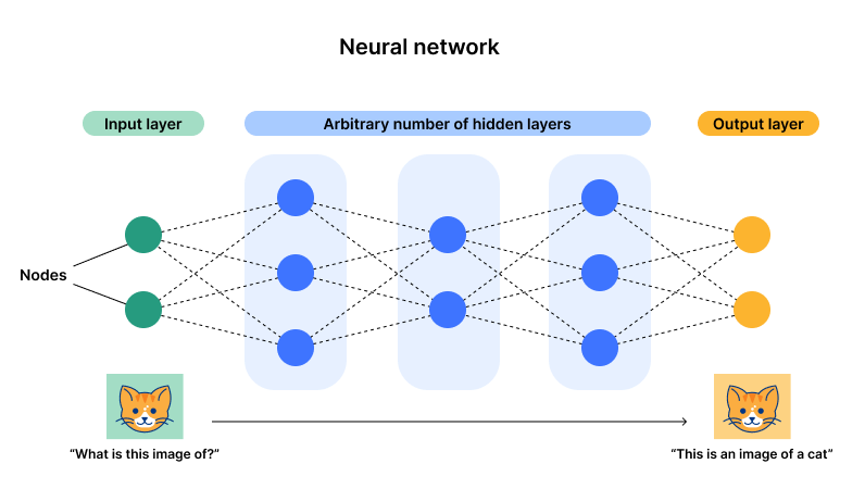
Reference of the image.

Here is how data flows through the network:

Each neuron processes an input and produces an output.
The output becomes the input for neurons in the next layer.
It repeats layer by layer till the last layer.
The last layer gives the network’s answer.

The key part is that each neuron isn’t just performing addition or multiplication. Still, a non-linear transformation, a more complex operation that involves non-linear relationships, enables the network to learn complex patterns such as “this combination of features means it’s a cat, not a dog”.

How neurons process information

Each neuron receives inputs, performs a calculation, and decides whether to pass information forward. This is how it happens:

Receive inputs: Takes numbers from previous neurons (or raw data if it’s the first layer).
Apply weights: Each input is multiplied by its corresponding weight (importance).
Calculate the total: Adds all the weighted inputs together.
Apply activation function: Transforms the sum using a special mathematical function.
Pass or block: If the result exceeds a threshold, it sends the output to the next layer; otherwise, it ignores it.

Think of it like the battery saver function in your phone; it monitors the battery percentage and analyzes your usage patterns (inputs), then calculates the urgency (sum), and decides whether to activate power-saving mode or stay in normal mode (activation function + threshold).

Example

Let’s imagine that a neuron decides whether to activate the battery saver mode:

Inputs:

🪫 Battery level below 20%: Yes = 1 or No = 0
📈 High power apps running: Yes = 1 or No = 0
🔌 Away from charger for 4+ hours: Yes = 1 or No = 0

Weights (importance of each factor):

Low battery level: weight = 0.6
High power apps: weight = 0.3
Time away from charger: weight = 0.4

Calculation:

Let’s say that for me, the battery level is 10%, I’m running high-power apps, and I’m away from my charger, so I’d say yes to all of the answers. Then we have to multiply the input value by the weight and sum all of them:

sum = (1 * 0.6) + (1 * 0.3) + (1 * 0.4)
sum = 1.3

Activation Function (simplified):

If sum > 1.0 → Output = 1 (activate battery saver!)
If sum ≤ 1.0 → Output = 0 (stay in normal mode)

Result:

In this example, the sum is 1.3 > 1.0, so the neuron fires (outputs a 1), triggering battery-saving mode to conserve power.

In the previous example, we saw that the activation function determines whether the battery saver should be turned on; in other words, let’s call this function the neuron’s decision maker! 😎

The Activation Function

The activation function is what makes neurons smart. Instead of just passing the sum directly, it transforms it into practical ways.

Common activation functions

Step function (simplest):

If sum > threshold → output 1
If sum ≤ threshold → output 0

Like a light switch; either ON or OFF.

Sigmoid Function (more sophisticated):

Output = 1 / (1 + e^(-sum))

Produces smooth values between 0 and 1, like a dimmer switch. Gives 0.5 when the sum is 0, values near 0 for negative sums, and values near 1 for positive sums.

ReLU (Rectified Linear Unit - most popular today):

If sum > 0 → output = sum
If sum ≤ 0 → output = 0

Passes positive values unchanged, blocks negative values. Simple but powerful 🦾

Visual Diagram

Neural Network Example

Now that we know how neurons process information, it’s essential to understand that there are different types of neural networks specialized for other tasks. In the next section, we’ll explore those types.

How Neural Networks Learn

So far, we’ve seen how neural networks process information, but how do they actually learn to make accurate predictions?

Neural networks learn through a process called training. Initially, the network’s weights are random, so the outputs are basically guesses. The network compares its output to the correct answer, calculates how wrong it was, the “error”, and then adjusts the weights slightly to reduce that error. This happens thousands or millions of times across the entire training dataset.

When you first try throwing a basketball, it’s kind of random where it goes. You look at how far off you were, maybe adjust your grip or the force of your throw, then try again. You keep doing that over and over until you start hitting the hoop pretty consistently.

The network works in a similar way. It looks at what it got wrong and tweaks things little by little to improve.

That tweaking part is called backpropagation, which means sending the error back through the layers. And the way it slowly gets better is called gradient descent, like going down toward less error.

In real setups, there are fancier methods like Adam that speed up training, but for now, sticking with basic gradient descent keeps things simpler. The main idea is that networks learn by changing their weights each time based on mistakes. They repeat that process a lot. We won’t dive into the math here, but understanding that networks learn by repeatedly adjusting weights based on their mistakes is crucial.

Wrapping up, the neural networks aren’t programmed with rules; they discover patterns by learning from examples.

Types of neural networks

There are different neural network architectures focused on various tasks. Understanding these types helps clarify why transformers became the foundation for modern LLMs, so considering their specialization, we have these types:

Feedforward Networks: The simplest architecture where information flows in one direction: input → hidden layers → output. No loops or backward connections.
Convolutional Neural Networks (CNNs): Specialized for processing grid-like data, especially images. CNNs detect patterns, such as edges, and combine them into more complex features, such as shapes and objects. They are focused on computer vision tasks, including face recognition, object identification, and medical image analysis.
Recurrent Neural Networks (RNNs): Created for sequential data where order matters, like time series, speech, or text. Unlike feedforward networks, RNNs have “memory”; they pass information from one step to the next, allowing them to remember previous inputs. However, they struggle with long sequences because their memory fades over time.
Transformer Models: The LLM Revolution; this is where things get interesting for LLMs. Transformers solved RNNs’ most significant limitation; they can process entire sequences simultaneously rather than one element at a time.

You can also see in some places that existing types like Perceptron, Multilayer Perceptron, Modular, Radial Basis, etc., but to mention, this classification focuses on how neurons are connected and organized, basically by their architecture.

Transformer model

The innovation in this model is that, unlike RNNs, which process text word by word, transformers can attend to all words at once and understand relationships between distant words, for example, in this sentence, “The dog didn’t run anymore because it was too tired.”, a transformer instantly connects “it” back to “dog”, even though they’re separated by several words.

This parallel processing makes transformers:

Faster to train than RNNs (can process all words simultaneously)
Better at understanding context (attention mechanism captures long-range dependencies)
More scalable (can be trained on massive datasets efficiently)

LLMs like ChatGPT and Claude use transformer architecture because it shines at understanding language patterns, maintaining context across long conversations, and generating coherent, contextually relevant text.

Putting It All Together

Before moving to the last section, let’s recap what we’ve learned:

Machine Learning teaches computers to learn patterns from data instead of following hardcoded rules.
Deep Learning uses multi-layered neural networks to discover features at different levels of abstraction automatically.
Neural networks are built from individual neurons that receive inputs, apply weights, sum everything up, pass the result through an activation function, and output a signal. Different types, such as CNNs, RNNs, and transformers, focus on various tasks, with transformers revolutionizing language understanding and powering modern LLMs.

Now that you understand the theory, let’s jump to the funniest part. Building a neural network in Ruby sounds kind of exciting, actually. Like doing it all from scratch without any of those frameworks or anything fancy, just straight Ruby code.

You’ll create neurons, connect them into a network, and watch it learn to solve a problem. This hands-on experience will solidify everything you’ve learned and prepare you for the advanced AI features we’ll build in Rails applications throughout this series.

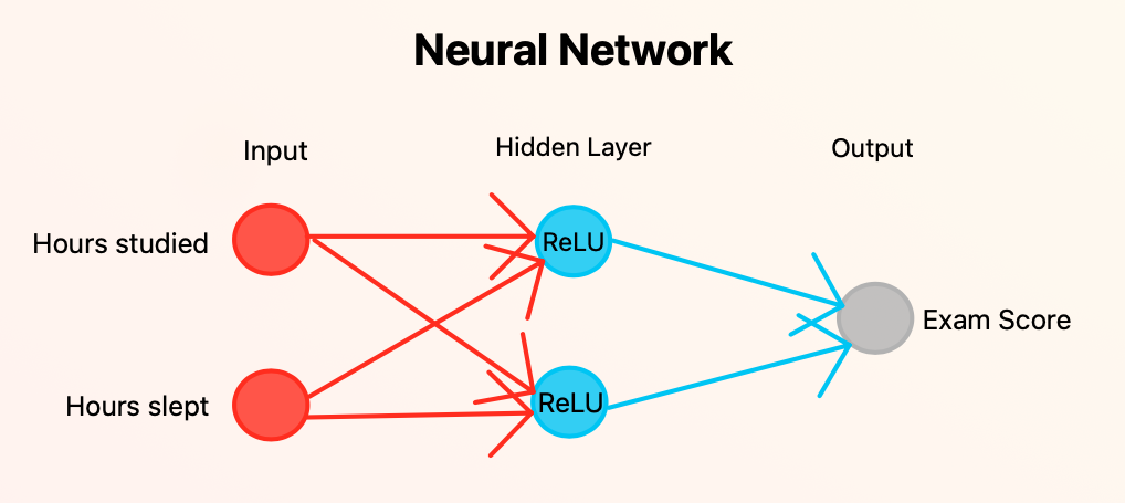
Practical Example: Predicting Student Test Scores

Let’s build a neural network that predicts a student’s final exam score based on:

Hours studied
Hours slept

We will have 2 inputs (hours studied and hours slept), 2 hidden neurons (using ReLU), and 1 output (exam score). This is a diagram to understand the architecture of our neural network:

Neural Network Architecture

To start with the Ruby script, let’s create a file such as predicting_student_test_scores.rb then let’s go to the funniest part:

As we saw before, a neural network starts with the training, and to do that, we need some training data:

# Training data: [hours_studied, hours_slept] → exam_score
training_data = [
  [[5, 8], 85], # 5 hours studied, 8 hours slept → 85 score
  [[2, 6], 60], # 2 hours studied, 6 hours slept → 60 score
  [[8, 7], 95]  # 8 hours studied, 7 hours slept → 95 score
]

Then, we need something called hyperparameters, which are helpful because we have to tell the network:

How big are the steps when updating weights? - Learning rate
How many times do we go through the entire training dataset? - Epochs

# Hyperparameters
learning_rate = 0.0001
epochs = 1000

Remember that:

Learning rate: A small value is equal to slow but stable learning.
Epochs: More epochs are equal to more opportunities to learn.

Later, we will see that when the learning rate is too large (0.01 or 0.1), the loss rate tends to increase instead of decrease, and the training becomes unstable.

Let’s continue. Now it’s time to initialize the weights and biases:

# Initialize random weights and biases
w1 = [[0.4, 0.6], [0.3, -0.2]]   # Weights from inputs to hidden layer (2x2)
w2 = [[0.8], [0.5]]              # Weights from hidden layer to output (2x1)
b1 = [0.5, -0.1]                 # Biases for hidden neurons
b2 = [10.0]                      # Bias for output neuron

These are random starting values. The network will adjust them during training.

Then, let’s create the ReLU Activation Function, which introduces non-linearity, allowing the network to learn complex patterns.

def relu(sum)
  [0, sum].max  # If sum is negative, return 0; otherwise return sum
end

Now that we have defined the variables such as training data, weights, biases, learning rate, and epochs, we are gonna move to the training loop, the Forward Pass. For each training example, the network makes a prediction:

# Training loop
puts 'Starting training...'
puts '-' * 50

epochs.times do |epoch|
  total_loss = 0

  training_data.each do |input, actual|
    # === FORWARD PASS ===
    # Hidden layer calculations

    # First hidden neuron (h1)
    # The weighted sum (z1) is also called linear combination or pre-activation
    z1 = (input[0] * w1[0][0]) + (input[1] * w1[1][0]) + b1[0]
    h1 = relu(z1)

    # Second hidden neuron (h2)
    z2 = (input[0] * w1[0][1]) + (input[1] * w1[1][1]) + b1[1]
    h2 = relu(z2)
    # ...
    # Don't close the epochs and training_data blocks yet

If we take the first training data example [5, 8], the weighted sum results are:

# Calculation results for the first training data example: [5, 8], w1 and b1
# because starts wiht the input → hidden layer
z1 = (5 * 0.4) + (8 * 0.3) + 0.5 = 4.9
h1 = 4.9

z2 = (5 * 0.6) + (8 * -0.2) + (-0.1) = 1.3
h2 = 1.3

Having the hidden neuron values, we can calculate the prediction for the output layer:

# We use w2 and b2 because goes from hidden layer → output
prediction = (h1 * w2[0][0]) + (h2 * w2[1][0]) + b2[0]

We can substitute with values:

prediction = (4.9 * 0.8) + (1.3 * 0.5) + 10 = 14.57

So, comparing our training data for [5, 8] the output of the exam score should be 85 but the newtwork predicted 14.57, which means we have a loss rate. Let’s calculate what that loss is:

# === CALCULATE LOSS ===

# Output layer error
error = prediction - actual

loss = error**2 # we square the error to get a positive number
total_loss += loss

And, the same, we replace with values:

# Actual is the output from our training data
error = 14.57 - 85
error = -70.43

loss = (-70.43)^2
loss = 4960.38

Our loss was about 4960.38 but the cool thing here is that our network learns about it, and we call this process backpropagation.

The next step is to start with backpropagation, where the network learns by calculating how much each weight contributed to the error. We have to calculate the gradients, and you’re probably wondering what they are here. A gradient tells us how much the loss would change if we changed a specific weight by a small amount.

Think of gradients as directions and magnitudes:

Direction (sign): Should we increase or decrease this weight?
- Positive gradient: decrease the weight.
- Negative gradient: increase the weight.
Magnitude (size): How much does this weight affect the error?
- Large gradient: this weight has a big impact on the error.
- Small gradient: this weight has minimal impact

Wrapping up how we can see the results:

Negative error means we predicted too low, so we need to increase the output
Positive error means we predicted too high, so we need to decrease the output

# === BACKPROPAGATION ===

# Gradients for w2 (Hidden → Output)
grad_hidden1_to_output = error * h1
grad_hidden2_to_output = error * h2
grad_output_bias = error

# Propagate error back to hidden layer
error_h1 = error * w2[0][0] * (z1.positive? ? 1 : 0) # ReLU derivative
error_h2 = error * w2[1][0] * (z2.positive? ? 1 : 0)

# Gradients for w1 (Input → Hidden)
grad_studied_to_hidden1 = error_h1 * input[0]
grad_slept_to_hidden1 = error_h1 * input[1]
grad_studied_to_hidden2 = error_h2 * input[0]
grad_slept_to_hidden2 = error_h2 * input[1]
grad_hidden1_bias = error_h1
grad_hidden2_bias = error_h2

And the results are:

# Gradients for w2 (Hidden → Output)
grad_hidden1_to_output = (-70.43) * 4.9 = -345.11
grad_hidden2_to_output = (-70.43) * 1.3 = -91.56
grad_output_bias = -70.43

# Propagate error back to hidden layer
error_h1 = (-70.43) * 0.8 * 1 = -56.34
error_h2 = (-70.43) * 0.5 * 1 = -35.22

# Gradients for w1 (Input → Hidden)
grad_studied_to_hidden1 = (-56.34) * 5 = -281.7
grad_slept_to_hidden1 = (-56.34) * 8 = -450.72
grad_studied_to_hidden2 = (-35.22) * 5 = -176.1
grad_slept_to_hidden2 = (-35.22) * 8 = -281.76
grad_hidden1_bias = -56.34
grad_hidden2_bias = -35.22

These calculate how much each input weight contributed to the error.

Once we have calculated the gradients, we need to update the weights using those gradients. We will use an optimization algorithm called SGD (Stochastic Gradient Descent), which is the primary optimization algorithm for training neural networks. It updates weights using a single data sample at a time instead of the entire dataset, making it fast and scalable:

  # === UPDATE WEIGHTS (SGD) ===

  # Update w2 (Hidden → Output)
  w2[0][0] -= learning_rate * grad_hidden1_to_output
  w2[1][0] -= learning_rate * grad_hidden2_to_output
  b2[0] -= learning_rate * grad_output_bias

  # Update w1 (Input → Hidden)
  w1[0][0] -= learning_rate * grad_studied_to_hidden1
  w1[1][0] -= learning_rate * grad_slept_to_hidden1
  w1[0][1] -= learning_rate * grad_studied_to_hidden2
  w1[1][1] -= learning_rate * grad_slept_to_hidden2
  b1[0] -= learning_rate * grad_hidden1_bias
  b1[1] -= learning_rate * grad_hidden2_bias
end # Close the training_data.each block

If we replace with the real values, we can see:

# Calculations for w2
w2[0][0] = 0.8 - (0.0001 * -345.11) = 0.8 + 0.0345 = 0.8345
w2[1][0] = 0.5 - (0.0001 * -91.56) = 0.5 + 0.0092 = 0.5092
b2[0] = 10.0 - (0.0001 * -70.43) = 10.0 + 0.0070 = 10.007

# Calculations for w1
w1[0][0] = 0.4 - (0.0001 * -281.7) = 0.4 + 0.0282 = 0.4282
w1[1][0] = 0.3 - (0.0001 * -450.72) = 0.3 + 0.0451 = 0.3451
w1[0][1] = 0.6 - (0.0001 * -176.1) = 0.6 + 0.0176 = 0.6176
w1[1][1] = -0.2 - (0.0001 * -281.76) = -0.2 + 0.0282 = -0.1718
b1[0] = 0.5 - (0.0001 * -56.34) = 0.5 + 0.0056 = 0.5056
b1[1] = -0.1 - (0.0001 * -35.22) = -0.1 + 0.0035 = -0.0965

We subtract learning_rate * gradient from each weight. This encourages the weights in the direction that reduces error. Notice that all weights increased because the error was negative, which means we predicted too low; if you remember, our prediction was 14.57 out of 85.

Let’s monitor the progress:

end # Close the training_data.each block

  # Calculate average loss
  avg_loss = total_loss / training_data.length

  # Print progress every 100 epochs
  puts "Epoch #{epoch + 1}: Avg Loss = #{avg_loss.round(2)}" if ((epoch + 1) % 100).zero?
end # Close the epochs.times block

Every 100 epochs, print the average loss. You should see this number decrease over time as the network learns.

Finally, to see all the complete training with some test cases, let’s add this:

puts '-' * 50
puts 'Training complete!'
puts

# === FINAL WEIGHTS ===
puts 'Final weights:'
puts 'w1 (Input → Hidden):'
puts "  Hours studied → H1: #{w1[0][0].round(3)}, H2: #{w1[0][1].round(3)}"
puts "  Hours slept → H1: #{w1[1][0].round(3)}, H2: #{w1[1][1].round(3)}"
puts 'w2 (Hidden → Output):'
puts "  H1 → Score: #{w2[0][0].round(3)}"
puts "  H2 → Score: #{w2[1][0].round(3)}"
puts "Biases: b1 = [#{b1[0].round(3)}, #{b1[1].round(3)}], b2 = [#{b2[0].round(3)}]"
puts

# === TEST THE NETWORK ===
puts 'Testing the trained network:'
puts '-' * 50

test_cases = [
  [5, 8],  # Original training example
  [2, 6],  # Original training example
  [8, 7],  # Original training example
  [6, 7],  # New student
  [3, 5],  # Low effort
  [9, 8]   # High effort
]

test_cases.each do |input|
  # Forward pass
  z1 = (input[0] * w1[0][0]) + (input[1] * w1[1][0]) + b1[0]
  h1 = relu(z1)

  z2 = (input[0] * w1[0][1]) + (input[1] * w1[1][1]) + b1[1]
  h2 = relu(z2)

  prediction = (h1 * w2[0][0]) + (h2 * w2[1][0]) + b2[0]

  puts "Input: [studied: #{input[0]}h, slept: #{input[1]}h] → Predicted score: #{prediction.round(1)}"
end

Running the Ruby script, you should see something like this:

> ruby predicting_student_test_scores.rb

Starting training...
--------------------------------------------------
Epoch 100: Avg Loss = 1.59
Epoch 200: Avg Loss = 0.96
Epoch 300: Avg Loss = 0.85
Epoch 400: Avg Loss = 0.83
Epoch 500: Avg Loss = 0.83
Epoch 600: Avg Loss = 0.82
Epoch 700: Avg Loss = 0.82
Epoch 800: Avg Loss = 0.81
Epoch 900: Avg Loss = 0.81
Epoch 1000: Avg Loss = 0.8
--------------------------------------------------
Training complete!

Final weights:
w1 (Input → Hidden):
  Hours studied → H1: 1.336, H2: 1.122
  Hours slept → H1: 2.021, H2: 0.739
w2 (Hidden → Output):
  H1 → Score: 2.581
  H2 → Score: 1.28
Biases: b1 = [0.824, 0.073], b2 = [10.193]

Testing the trained network:
--------------------------------------------------
Input: [studied: 5h, slept: 8h] → Predicted score: 86.1
Input: [studied: 2h, slept: 6h] → Predicted score: 59.2
Input: [studied: 8h, slept: 7h] → Predicted score: 94.6
Input: [studied: 6h, slept: 7h] → Predicted score: 84.9
Input: [studied: 3h, slept: 5h] → Predicted score: 57.9
Input: [studied: 9h, slept: 8h] → Predicted score: 105.7

We can notice that the average loss is decreasing on each iteration. Even if you want to see how the loss is changing, we just need to print every 50 epochs:

> ruby predicting_student_test_scores.rb

Starting training...
--------------------------------------------------
Epoch 50: Avg Loss = 2.68
Epoch 100: Avg Loss = 1.59
Epoch 150: Avg Loss = 1.14
Epoch 200: Avg Loss = 0.96
Epoch 250: Avg Loss = 0.88
Epoch 300: Avg Loss = 0.85
Epoch 350: Avg Loss = 0.84
Epoch 400: Avg Loss = 0.83
Epoch 450: Avg Loss = 0.83
Epoch 500: Avg Loss = 0.83
Epoch 550: Avg Loss = 0.83
Epoch 600: Avg Loss = 0.82
Epoch 650: Avg Loss = 0.82
Epoch 700: Avg Loss = 0.82
Epoch 750: Avg Loss = 0.81
Epoch 800: Avg Loss = 0.81
Epoch 850: Avg Loss = 0.81
Epoch 900: Avg Loss = 0.81
Epoch 950: Avg Loss = 0.8
Epoch 1000: Avg Loss = 0.8
--------------------------------------------------
Training complete!

Finally, let’s see how changing the learning rate to a bigger number, increase the average loss, so we have to update the learning_rate to 0.01 and run the script:

> ruby predicting_student_test_scores.rb

Starting training...
--------------------------------------------------
Epoch 50: Avg Loss = 482.11
Epoch 100: Avg Loss = 231.57
Epoch 150: Avg Loss = 219.43
Epoch 200: Avg Loss = 218.87
Epoch 250: Avg Loss = 218.85
Epoch 300: Avg Loss = 218.85
Epoch 350: Avg Loss = 218.85
Epoch 400: Avg Loss = 218.85
Epoch 450: Avg Loss = 218.85
Epoch 500: Avg Loss = 218.85
Epoch 550: Avg Loss = 218.85
Epoch 600: Avg Loss = 218.85
Epoch 650: Avg Loss = 218.85
Epoch 700: Avg Loss = 218.85
Epoch 750: Avg Loss = 218.85
Epoch 800: Avg Loss = 218.85
Epoch 850: Avg Loss = 218.85
Epoch 900: Avg Loss = 218.85
Epoch 950: Avg Loss = 218.85
Epoch 1000: Avg Loss = 218.85
--------------------------------------------------
Training complete!

Final weights:
w1 (Input → Hidden):
  Hours studied → H1: -8.216, H2: -1.446
  Hours slept → H1: -29.491, H2: -8.804
w2 (Hidden → Output):
  H1 → Score: -44.62
  H2 → Score: -26.389
Biases: b1 = [-4.653, -1.651], b2 = [80.034]

Testing the trained network:
--------------------------------------------------
Input: [studied: 5h, slept: 8h] → Predicted score: 80.0
Input: [studied: 2h, slept: 6h] → Predicted score: 80.0
Input: [studied: 8h, slept: 7h] → Predicted score: 80.0
Input: [studied: 6h, slept: 7h] → Predicted score: 80.0
Input: [studied: 3h, slept: 5h] → Predicted score: 80.0
Input: [studied: 9h, slept: 8h] → Predicted score: 80.0

The average loss is bigger and it didn’t decrease affecting the predictions, so that’s the reason a small learning rate is better.

You can check the whole code in this repository!

Summary of the Learning Process

Forward Pass: Make a prediction
Calculate Error: Compare prediction to actual value
Backpropagation: Calculate how much each weight contributed to the error
Update Weights: Adjust weights to reduce error
Repeat: Do this 1000 times across all training examples

After 1000 epochs, the network should have learned that more studying and more sleep lead to higher test scores!

Key Insights

First prediction was 14.57, target was 85, so huge error of -70.43.
All weights increased because the error was negative (prediction too low).
A small learning rate (0.0001) means weights change slowly but steadily.
After 1000 epochs, these small adjustments accumulate, and the network learns!

The network will repeat this process with all 3 training examples 1000 times, gradually adjusting the weights until the predictions become accurate.

Conclusion

With this example, we’ve completed the first essential step in understanding the foundations of LLMs. You’ve learned the core concepts of Machine Learning and Deep Learning, and most importantly, you’ve built a working neural network from scratch in Ruby. This hands-on experience with neurons, weights, and backpropagation gives you the knowledge needed to understand how modern AI systems work under the hood.

In the next posts, we’ll integrate AI capabilities into Rails applications, moving from theory to building real-world features. Stay tuned! 👋

Tags: ruby AI neurons neural-network machine-learning deep-learning